Here is image of tanh (hyperbolic tangent) function from Gnuplot37, overlaid with hypertanf sAPL function from "neuralxr" workspace. This sAPL workspace will accept the MNnet4~1.WTT file of Xerion weights for the MarketNet network, and use dot-product to vector multiply the weights to "activate" the Xerion-trained network. This will let me "run" the network, on the iPad. I wrote the function to load the Xerion weights file into sAPL, (format: wt <- readfile fname) and second function to convert the text into numeric (format: wnet <- procwt wt). Currently, wnet is just a high-precision vector of 1281 32-bit floats. Since I'm using hyperbolic tangent instead of logistic as my transfer function, I needed to write this tiny transfer function. The tanh function already exists in GNUplot37. You can start GNUplot, and just enter "plot tanh(x)" and see this S-curve, which is the mechanism by which machine-intelligence is stored in a neural-network. Getting closer for an NN-based iPad-runable Augmenter. [Update: I wrote the function on top-left, but then remembered the APL built-in trig. functions, and yes, "7oX" gives hyperbolic tangent for X. The "o" operator is "ALT-o", and when used dyadic (two arguments), it gives access to all the trig. functions. With full precision of 18 digits enabled, the built-in "tanh" function gives slightly more precise results.]

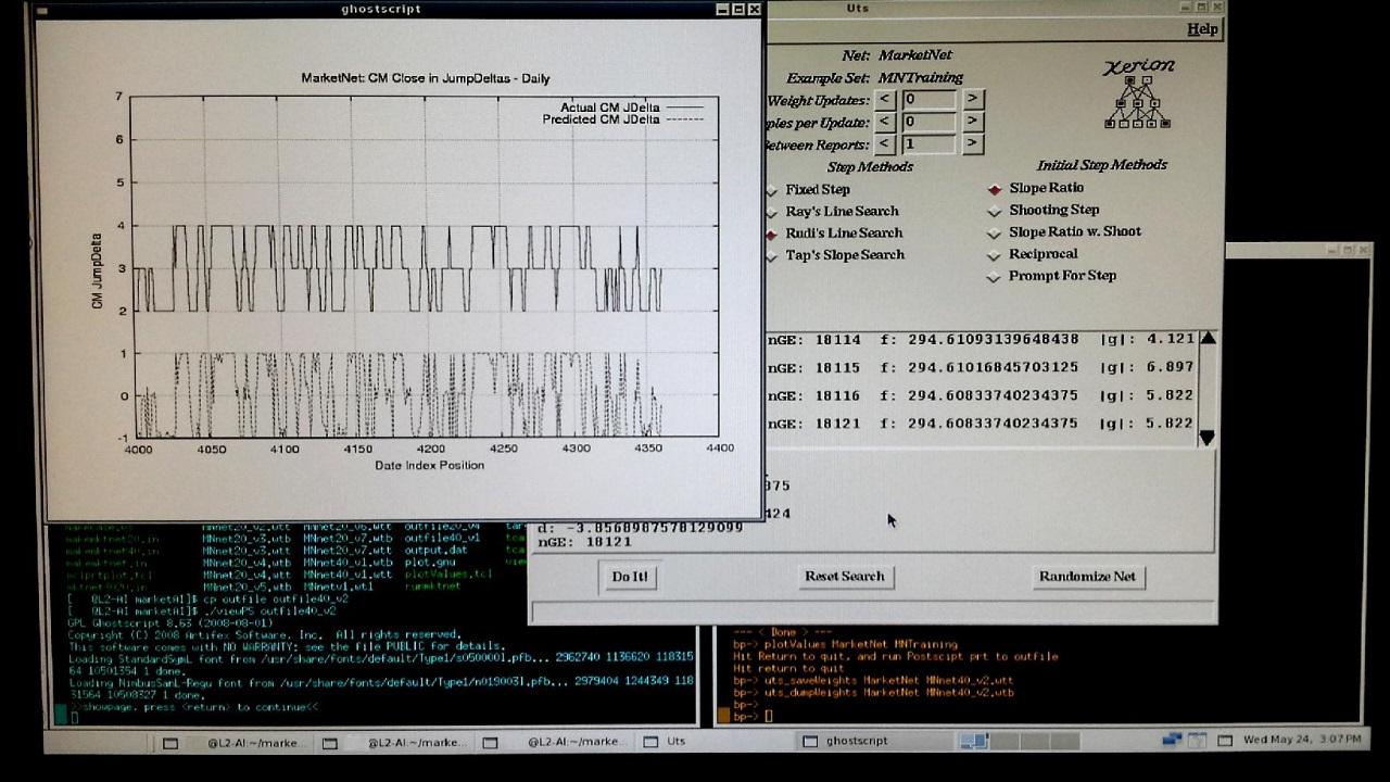
This screen shot from the Linux AI-box is a quick way to post results - not sophisticated, but clear. Speaking of "quick", I used the "quickProp" method here, which models derivatives as independent quadratics. The method tries to jump to the projected minimum of each quadratic. This is one of the minimization methods in Xerion, and it has worked well on my signed boolean data. (See: S. Fahlman "An Empirical Study of Learning Speed in Back-Propagation Networks", 1988, CMU-CS-88-162, Carnegie-Mellon University.) Typically this method uses fixed steps with epsilon of 1, but I used a line-search here. The error value (f:) is driven down below 300, with a gradient vector length of less than 6. From the plotValues.tcl chart, one can see it improves on the previous result. If this network is this good on a different dataset outside the training example, then we might just have something here. I want to thank Dr. Hinton and everyone at U of Toronto for making Xerion available.

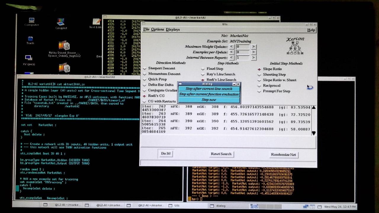
Running Xerion with gui, running backpropagation using conjugate gradient and line-search, with new network with twice the nodes. Error level (F:) down below previous 20 node network in less than 400 evaluations. Looks good - works well.

[Initial Results: - MarketNet was built using signed boolean jump coding. Note that for the graphic (Postscript output, shown using GhostView), I tweaked my plotValues.tcl displayer to shift the actual data +3 up, so it does not obscure the network output forecast. The network is called "MarketNet", and is not fully trained, as I need to reset the "tcl_precision" value to 17 (from its default of 6). With improved precision, the network trains further, and should become more accurate. What one needs to do, is save the weights, and then try the network on a dataset built for a different time period. This will provide indication of whether I am just training to noise or not.]